How To Do Pie Chart In Excel

If we choose to make a 3D pie chart it will look like this. Right click the pie chart again and select Format Data Labels from the right-clicking menu. Lets see how to create Pie of Pie chart in Excel.

lords mobile monster hunt chart bmi chart in kg john paul jones seating chart bra sizes measurement chart ariat tall boot size chart the chart of accounts is a org chart in powerpoint ak chin pavilion seating chart

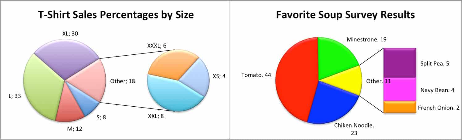
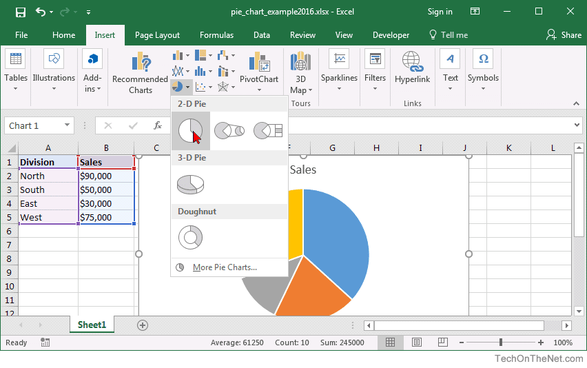
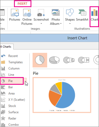
Select the data click Insert tab chose pie chart ribbon Pie of pie chart as shown below.

How to do pie chart in excel. In the Charts group click on the Insert Pie or Doughnut Chart icon. Select the data range in this example B5C14. How do you add descriptive.

To create a pie chart in Excel 2016 add your data set to a worksheet and highlight it. How do I change the colors of a pie chart in Excel 2007. If you forget which button is which hover over each one and Excel will tell you which type of chart it is.

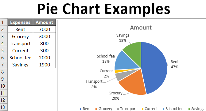
Click the chart and then click the icons next to the chart to add finishing touches. First we select the data we want to graph. Just like any chart we can easily create a pie chart in Excel version 2013 2010 or lower.

On the Format tab in the Current Selection group click Format Selection. Click on the Bar of Pie chart icon within 2-D Pie icons. In this case the chart we want is this one.

On the Insert tab in the Charts group choose the Pie and Doughnut button. In your spreadsheet select the data to use for your pie chart. Then click the Insert tab and click the dropdown menu next to the image of a pie chart.

Open the document containing the data that youd like to make a pie chart with. Click and drag to highlight all of the cells in the row or column with data that you want included in your pie graph. To create a Pie of Pie or Bar of Pie chart follow these steps.

Pie Exploded Pie Pie of pie Bar of pie or 3D pie chart. Open the document containing the data that youd like to make a pie chart with. Select the entire data set.

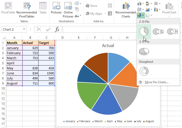
Pie of Pie chart in Excel Step 2. Tab expand Fill and then do one of the following. In the resulting menu click 2D Pie.

So our chart will be like. Click the Insert tab. How to create a pie chart.

Kasper Langmann Co-founder of Spreadsheeto. How do I make a pie chart in Excel from one column. How do I make a pie chart in Excel from one column.

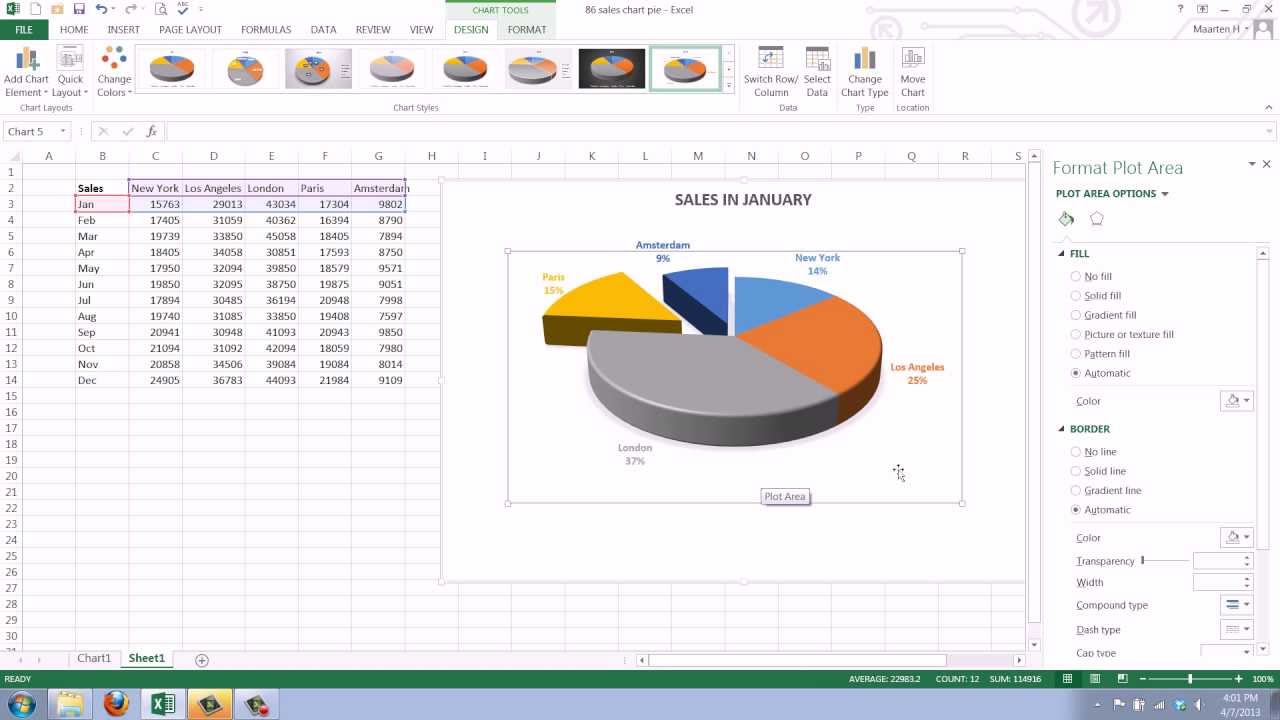
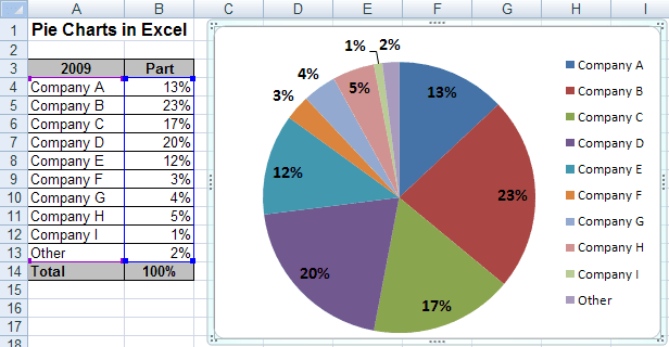
In the opening Format Data Labels pane check the Percentage box and uncheck the Value box in the Label Options section. Click the Insert tab at the top of the screen then click on the pie chart icon which looks like a pie chart. Click Insert tab Pie button then choose from the selection of pie chart types.

Click the Insert tab at the top of the screen then click on the pie chart icon which looks like a pie chart. How do you make a 3 D pie chart in Excel. Select the data click Insert click Charts and then choose the chart style you want.

Click and drag to highlight all of the cells in the row or column with data that you want included in your pie graph. Then click to the Insert tab on the Ribbon. Each of these chart sub-types separates the smaller slices from the main pie chart and displays them in a supplementary pie or stacked bar chart.

Click Insert Insert Pie or Doughnut Chart and then pick the chart you want. Drawing a pip chart is the same as drawing almost any other chart. Then the percentages are shown in the pie chart as below screenshot shown.

Here are the steps to create a Pie of Pie chart. How do you make a. For more information about how pie chart data should be arranged see Data for pie charts.

In the Charts group click Insert Pie or Doughnut Chart. To vary the colors of data markers in a single-series chart select the Vary colors by point check box. How do I create a percentage pie chart in Excel.

In a chart click to select the data series for which you want to change the colors. Pie of Pie chart in Excel Step 1. From the chart styles chose the style of charts that suits our representation.

Select the chart type you want to use and the chosen chart will appear on the worksheet with the data you selected. Pie of Pie chart in Excel Step 3.